Measure of Dispersion

Share/Comment
	Tweet		Facebook
	Feedback		EMail

Let us first take a closer look at dispersion. Here are two frequency distribution graphs drawn from two different data sets of pizza delivery time.

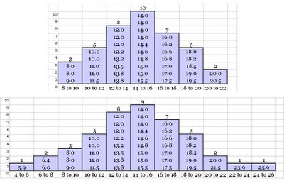
Notice both have a mean value of 14.4, but the degree of spread or scatter are different. The second data set has a higher spread compared to the first one. In other words, the second one has higher variability. Recall, one of the key objective in Six Sigma is to reduce variation. Therefore, it is very important to understand different key measures of dispersion clearly.

Range

It is the difference between the highest and the lowest value in the data set. In our first data set of pizza shop example, it is (20.5-8.0) or 12.5 whereas in the second case it is (25.9 - 5.9) or 20.0.

Interquartile Range

As the name suggest, it is the range of middle 50% of the ordered data set. Let us look at the pizza shop example data again. The interquartile range in the first case is (16.8 - 12.0) = 4.8, and in the second case it is (17.0 - 12.0) = 5.0.

Clearly, interquartile range is less impacted by the extreme values of the data set, as compared to the range. However, both fail to provide an average figure of deviation or scatter present in the dataset.

Standard Deviation - Measure of Average Deviation

One simple way to determine average deviation seems to be to find the average of the expression (mean - data value) for every data value in the data set.

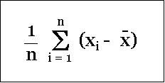
But there is a catch! It will be virtually "0". You may like to try it with one of the example data set given above.

So, how do we compute average deviation? A smart idea would be to find average of the absolute value of the expression (mean - data value) for every data value in the data set. Note, absolute value means ignoring the "-" sign.

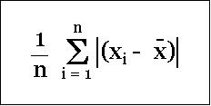
This quantity is referred as Mean Absolute Deviation (MAD). MAD for the first data set is 2.6 and for the second data set is 3.3. This appears to be a good average measure of deviation. But, still there is a problem. Here the larger deviation values tend to get averaged out and the value does not reflect the impact of larger scatter or dispersion properly.

Therefore, it will be appropriate to compute root mean square (RMS) of deviations (from the mean) instead of the simple mean. RMS is the square root of the mean of square of the each data value.

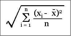
Since, each data value is squared, the larger values automatically get amplified accordingly to reflect the impact of larger deviations. To understand the concept, let us look at the following data and the corresponding graph.

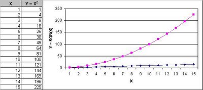
The data shows X and Y values, where Y value is the square of X value. In the graph, the dark blue line represents the X value and the pink line represents the Y value. Notice how Y becomes increasingly larger with increase in X value. This means the large the deviation translates to correspondingly larger impact (i.e. the effect of squaring). Therefore, RMS is a faithful measure of average deviation. This is what is known as Standard Deviation.

Here are the details of the first data set that we can use to quickly compute the vales ourselves.

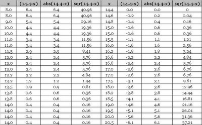
The Standards Deviation for the first data set is 3.2 and for the second data set is 4.4. Notice the affect of the amplification of larger scatter in the second case (i.e. 2.6 & 3.2 versus 3.3 & 4.4). Following table illustrates the mathematical formula for population standard deviation.

Following table illustrates the mathematical formula for sample standard deviation. The reason for division by "(n - 1)" instead of "n" is discussed later.

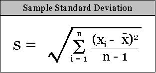
Variance

The square of standard deviation is known as Variance. Why did we need to define one more parameter, when standard deviation appears to be the right answer? It has some interesting and useful properties. Prominent one is the addition property for two independent data sets or observations. In other words, variance of the sum of independent data sets or observations (also referred random variables) is the sum of their variances.

Coefficient of Variation

Having discovered a good measure of average deviation, how do we compare the spread or scatter of two independent data sets? Just knowledge of standard deviation is not enough - it is the absolute measure of average deviation of a data set. For the purpose of comparison, we need to look at both mean and standard deviation together. Coefficient of Variation does that precisely.

Let us take an example. Consider two different data sets having mean and standard deviation as "14.4 & 3.2" and "144.0 & 3.2" respectively. The same standard deviation does not mean identical degree of scatter. In fact the second one has very little degree of spread or scatter. And coefficient of variation highlights it clearly - coefficient of variation for the first data set is 22.2 and for the second data set it is 2.2.

Z-Score

The z score of a data point or observation indicates how far and in what direction that observation is away from its data set's mean.

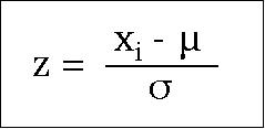
Z-score is revisited later in the section on distribution.

Commenting Guidelines
We hope the conversations that take place on “discover6sigma.org” will be constructive in context of the topic. To ensure the quality of the discussion stays in check, our moderators will review all the comments and may edit them for clarity and relevance. The comments that are posted using fowl language, promotional phrases and are not relevant in the said context, may be deleted as per moderators discretion. By posting a comment here, you agree to give “discover6sigma.org” the rights to use the contents of your comments anywhere.