So, where is the information?

Share/Comment
	Tweet		Facebook
	Feedback		EMail

We have drawn so many graphs. We have covered tons of mathematics - mean, mode, median, and MAD. But where is the information? When we look at mean of a data set, what do we understand from it? It is now time to see the unseen!

Let us begin with an example. Imagine that we are reviewing the production performance of our plants for last 30 days. The production managers are sharing the production details. John reports that the average production was 357287 units per day and his plant produced over 714213 units per day for 16 days in a row, which is a record. The production figures for all other managers were between 345623 and 366543 units per day. Does this tell us something? Think! Yes, it tells us a lot. What John reported is impossible. Let us do the mathematics to uncover that. Total production for John's plant is "357287 average units per day" x "30 days" = "10718610 units" and with 714213 x 16 the production figure during record period is 11427408 units. Impossible, isn't it?

Let us put our observation formally now. If the mean of a data set containing non negative numbers is "μ", then the percentage of observations or data points that are greater or equal to a value x is always smaller or equal to "100 * (μ/x)". This is called Markov's Inequality.

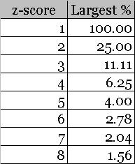
There is one more inequality worth learning. It is called Chebychev's Inequality. The largest percentage of values for a data set, that have a z score beyond "z" in either direction, is "100/(square of z)". The following table summarizes the outcome of this inequality for quick reference.

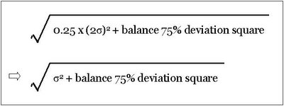
To understand this inequality, let us pick up any row from the above table - say the second row. Now assume, that there is a dataset having a mean of μ and standard deviation of σ. There are 25% values from the data set that are exactly 2σ away from the mean i.e. μ. With this knowledge at hand, we can write down the value of standard deviation as:

In order to arrive at the value of standard deviation as "σ", the second term must be "0" i.e. the balance 75% terms should be at mean. We can clearly see that it is not possible to have more than 25% values from the data set that are 2σ away from the mean.

Please note, that it applies to any distribution. At this stage, we may like to compare these figures with what we learned about normal distribution in Introduction to Six Sigma.

Let us revisit our famous pizza shop. The shop management wishes to add another area for pizza delivery. They collect information (read mean & standard deviation) on travel time for different routes over a period of time. This can now be used to perform a quick go/no-go analysis. Right?

Indeed, mean and standard deviation contains a lot of information that we can use in real life.

Commenting Guidelines
We hope the conversations that take place on “discover6sigma.org” will be constructive in context of the topic. To ensure the quality of the discussion stays in check, our moderators will review all the comments and may edit them for clarity and relevance. The comments that are posted using fowl language, promotional phrases and are not relevant in the said context, may be deleted as per moderators discretion. By posting a comment here, you agree to give “discover6sigma.org” the rights to use the contents of your comments anywhere.