| Share/Comment | |||
 |
Tweet |  |
|
 |
Feedback |  |
|
As discussed earlier, distribution tells us how data elements of a given data set are distributed within its range. It is time now to take a bigger bite into distribution and go beyond pizza delivery data.
Before we delve deeper into distribution, let us quickly revisit why it is important for us? Recall from Variation & Defect, "the natural variation always occurs and it can not be traced to a specific cause. It is random within a predictable range or in other words, it follows a distribution pattern".
It is really interesting to note that although each outcome of a random event is uncertain when seen in isolation; but collectively they follow a predictable pattern. This pattern is called its distribution function. Let us take an example to understand the concept - tossing an unbiased coin. What is the probability of getting a heads when we toss a coin? It is 0.5. What will happen if we toss the coin 20 times (we refer to this as an experiment)? Again the expectation is to get heads 10 times. Note it is only the expectation or the probability. The actual result may vary every time we repeat this experiment. Let us now repeat this experiment 20 times and note the distribution of observing heads in each experiment.
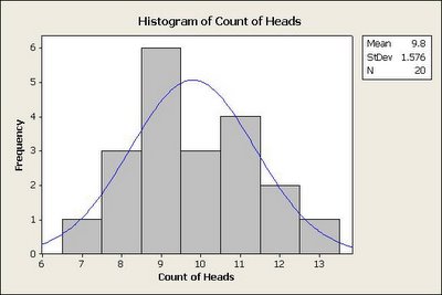
The following 2 graphs illustrate the distribution for the same experiment repeated 200 times and 2000 times respectively.
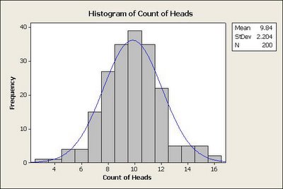
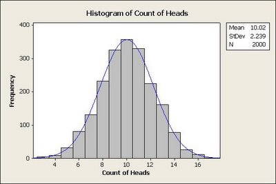
What do we observe from the above experiments? Something that we mentioned in the beginning - "collectively outcome of random events follow a predictable pattern". It becomes more evident with increasing number of experiments. The other key point to note is that the mean observed is also close to 10.
The graphs shown above are created using random data generated using MINITAB - a statistical software. However, It is strongly recommended to try this experiment manually by repeating it 10 times to get a practical feeling.
With this picture, it is time to look at the formal mathematical scenario. We will begin with binomial distribution.
Binomial Distribution
Suppose we toss a coin N-times. What will be probability of getting a specific sequence of "n" heads? This requires application of "Multiplication Rule for Independent Events". For further details, refer section on Basic Probability Theory. The probability is given by the following equation.
where "p" is the probability of getting heads.
If the sequence is not important then the probability will be determined by multiplying the above equation by NCn.
The above probability is the one that we observed empirically, when we conducted the "coin tossing" experiment. If you recall binomial theorem, it is very easy to observe that P(n, N) is the nth term of (p + (1 - p))N.
Brief Detour to Binomial Theorem
It tells us how to expand the power of sums. Let us look at the following simple expansions to develop a clear understanding.
(a + b)1 = a + b
(a + b)2 = a2 + 2ab + b2
(a + b)3 = a3 + 3a2b + 3ab2 + b3
(a + b)4 = a4 + 4a3b + 6a2b2 + 4ab3 + b4
A close observation of the above expansions reveals that each term in the expansion follows the formula for P(n, N). You must be wondering why the above expansions are written in a triangular manner. In fact, if you look at the coefficient of each term what you will see is the Pascal triangle. The same is illustrated below.
N = 1 1 1
N = 2 1 2 1
N = 3 1 3 3 1
N = 4 1 4 6 4 1
Pascal triangle provides us an easy way to find out each coefficient of term in the expansion.
Back to Binomial Distribution
The function to compute P(n, N) is called binomial distribution function. This function has some interesting characteristics. These are discussed below.
Binomial Distribution is Normalized
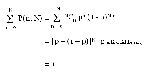
A normalized distribution function - "f(x)" must result into a sum of "1", if all values of "f(x)" for every "x" are added together. Such a function is also called probability distribution function (PDF). We can easily visualize by computing the sum of P(n, N) for every value of "n".
Mean of Binomial Distribution is N.p
Recall from Probability and Statistics, mean is the sum of product of "p(x)" and "x", for all values of "x". Therefore, in case of binomial distribution it can be computed using the following expression.
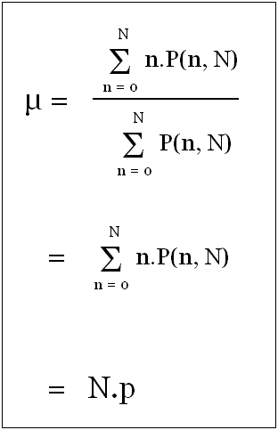
Although the rigorous mathematical proof is not given here, you are encouraged to try computing mean using simple values for "N" (e.g. 2 & 3).
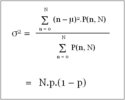
Variance of Binomial Distribution is N.p.(1-p)
The variance for binomial distribution can be computed using the following expression.
Example
Let us take an example for "N = 20" and "p = 0.5" to visualize the above characteristics. The following table shows the data. This data can be quickly constructed using a spreadsheet like MS Excel.
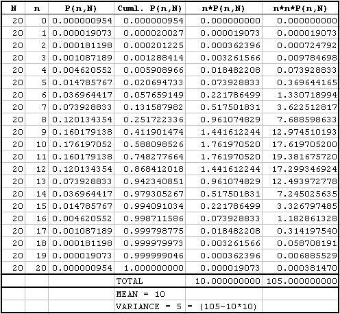
We can observe from cumulative P(n, N) column that the distribution is properly normalized as the last row has a value of "1". The mean and the variance are "10" and "5" respectively. Note, variance for grouped data is computed using ∑(fx² ⁄ N) − μ² formula. It can easily be seen that the expression ∑(fx² ⁄ N) is equal to n*n*P(n, N).
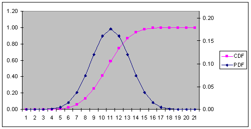
The above results also agree with our formula for mean and variance derived earlier. The following graphs illustrate the probability and cumulative distributions.
Binomial to Normal Distribution
Normal distribution can be approximated as a special case of binomial distribution for very large "N" and finite "p". Normal distribution is found in abundance in nature. Examples are covered in the topic on Distribution in Real Life later. The PDF of normal distribution is given below.
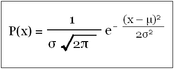
The "e" in the expression is called exponential function. It is expressed as "ex", where "e" is equal to approximately 2.7183. The concept of "e" will be discussed later.
Recall from Introduction to Six Sigma that 68% of area (i.e. the data points) falls within the area of -1σ and +1σ on either side of the mean. With this PDF, it is very easy to compute the area within +/- 1 σ from mean using the following expression.
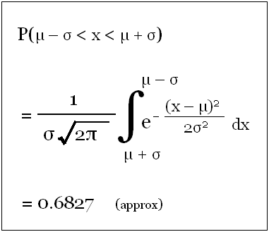
Other area computations can now be easily done using the same method.
At this stage we can also observe, how binomial distribution becomes normal distribution when N is very large and p has a finite value. We can compute the area under the binomial distribution with in +/- 1 σ for N=1000 & p=0.5. The expression for this calculation is given below.
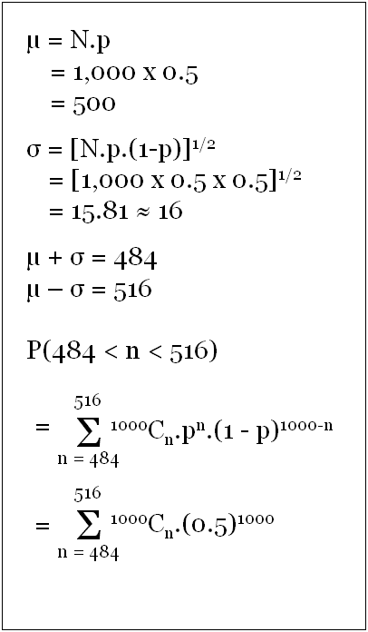
You will notice that this value will be approximately equal to 0.7, which is very close to 0.6827. This calculation can be carried out using any spreadsheet like MS Excel. As "N" becomes higher, this values approaches to 0.6827.
comments powered by Disqus
Commenting Guidelines
We hope the conversations that take place on “discover6sigma.org” will be constructive in context of the topic. To ensure the quality of the discussion stays in check, our moderators will review all the comments and may edit them for clarity and relevance.
The comments that are posted using fowl language, promotional phrases and are not relevant in the said context, may be deleted as per moderators discretion.
By posting a comment here, you agree to give “discover6sigma.org” the rights to use the contents of your comments anywhere.