| Share/Comment | |||
 |
Tweet |  |
|
 |
Feedback |  |
|
Equipped with basic knowledge of distribution, let us now explore the applications of distribution in our lives. A closer look will reveal that it has been used in cosmic world to quantum world to our daily lives. For example, astronomers studied the distribution of gamma ray bursts to predict the shape of our galaxy and the presence of stellar nurseries. In quantum physics, the Heisenberg's uncertainty principle also talks about the distribution of position of a particle or "delta x" - the uncertainty in position for a given uncertainty in momentum. A simpler example is heights of people - it follows a normal distribution - a natural phenomenon.
Real Life Applications
Let us look at some more real life applications.
Data Compression
A very common and easy to understand application is data compression. Almost all of us have used ZIP software at some point in time - right? Such software compresses the data by leveraging the distribution of letters or words contained in the data. Normally if you were to encode a message consisting of only English alphabets, you would assign a fixed 5-bits code to each alphabet irrespective of its distribution in the message to be encoded. The trick is to find out the distribution pattern of the alphabets and assign the shortest code to alphabet with highest frequency of occurrence and the longest to smallest frequency of occurrence. You can easily observe that this variable length encoding would lead to a compression compared to a fixed length encoding approach.
Reliability
In engineering world, reliability is defined as the probability that a system will function within its specified limits for a specified period of time under stated environmental conditions. We can easily visualize that reliability is all about studying the failure-time distribution under the given environmental conditions.
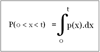
A quick and simple mathematical overview will add further clarity. Let us assume p(x) is the probability distribution function (PDF) of time to failure of a given component. The probability that the component will fail between a time interval of "0" and "t" will therefore be given by:

The reliability or the probability that the component will survive up to time t can easily be determined from the following equation.

Project Planning
Most common way of project planning is to identify the tasks required to complete the project, estimate their completion time, and determine their interdependencies followed by development of the network diagram (or graph) to compute project completion time along with other parameters. This methodology works well if (point) estimates of task completion time are highly accurate. In other words the actual completion time experiences negligible variation.
In real world that is full of variations, PERT methodology of project planning comes to our rescue. The 2 key differences in this methodology are (a) understanding the distribution of task completion time (from past data) and (b) application of Central Limit Theorem (CLT) to compute the project completion time with a defined confidence level.
The distribution of completion times provides us the minimum, maximum, and the most likely (mode) completion time, which allows us to compute the mean and variance of completion time. On the critical path of the project, the mean and variance are added to find out the mean project completion time and the corresponding variance. And this follows a normal distribution according to the CLT. With this information, we can now easily compute the project completion time with required confidence level. Imagine in case of point estimates equal to average task completion time value, the project completion time will have a confidence level of just about 50% only.
Quality Management
Conceptual understanding of distribution along with its practical applications is the foundation of several quality management techniques. These are discussed in detailed separately. Let us take a quick glimpse of its application. Let us say we receive a large shipment of certain part into our warehouse from the vendor. Vendor claims that there are no more than 2% defective parts in the shipment. If we sampled 150 parts randomly, what will be the probability of detecting at least one defective part? Simple application of binomial distribution will help us determine the answer. It will be 1 - P(n=0) and the value will be 0.95 approximately. For exact formula, please refer to binomial distribution in post on Distribution.
comments powered by Disqus
Commenting Guidelines
We hope the conversations that take place on “discover6sigma.org” will be constructive in context of the topic. To ensure the quality of the discussion stays in check, our moderators will review all the comments and may edit them for clarity and relevance.
The comments that are posted using fowl language, promotional phrases and are not relevant in the said context, may be deleted as per moderators discretion.
By posting a comment here, you agree to give “discover6sigma.org” the rights to use the contents of your comments anywhere.