Sampling

Share/Comment
	Tweet		Facebook
	Feedback		EMail

Do you remember the quote in the "first step" section of this site, "You can manage, what you can measure; you can measure, what you can define; you can define, what you can understand"? Operational definition was the first step towards effective management. It helps us build a clear understanding of a concept or a phenomenon so that it can be unambiguously measured.

The next step is measurement. Sampling is all about making measurement simpler, especially when you are required to take a large number of measurements. Let us take the example of our washer manufacturing process described in the post on Processes are everywhere. Imagine that this process is producing 100,000 washers every day. In order to ensure that washers shipped are within the specified tolerance limits, can we measure diameter of every washer before shipping? Probably not! It would be nice if we can pick up a representative sample consisting of few hundred washers, measure their diameter, and draw inference about the entire lot manufactured in a day. Sampling allows us to achieve this. At this stage, you may like to revisit the section on "Basic Statistics" in post on Statistics Simplified.

What is Sampling?

Sampling is a method to draw inference about one or more characteristics of a large group of items by examining a smaller but representative selection of group items. This selection is referred as the sample. This selection can be probability driven, or judgment/non-probability driven.

In non-probability sampling scheme, the probability of a population element being chosen is unknown and is based on the judgment of the researcher.

In probability driven sampling, each element of population has a "known non-zero" probability selection. It is easy to build mathematical or statistical models for drawing inference about the population. Our focus will be on this type of sampling.

One common example of probability sampling is "random sampling", where each element (and each combination of element) has an equal chance of being selected. More details are discussed later in this post.

Why Sampling?

Why can't we look at the entire population? Simply because sometimes the population is so large that it makes it prohibitive in terms of time and resources to carry out the measurements or survey. In any large volume manufacturing process, we face such challenges regularly. Other examples are exit polls, or any national level survey.

In addition, there are occasions where measurement leads to destruction of the item under consideration. Typical examples are measurement of tensile strength of a wire, or measuring battery life, or crash testing of a car.

Steps to Successful Sampling

The goal is to acquire a sample that is true representative of the population; it is something like a mini replica of population that is good enough to draw inference with required "accuracy & precision" about the population. Any successful sampling requires striking a balance between the required "accuracy & precision" and the "available resources". The key steps are outlined below.

1. Defining the population
2. Determining the sample size
3. Selecting the sampling technique

Defining the population

This is an important step if the entire population is not accessible for sampling. Ideal situation will be to draw sample from across the entire population. However, this may not be practical in every situation. The items within a population who can be sampled are usually limited. Such a target population, which can be sampled, is called a sampling frame. Defining this sampling frame is the first step of any successful sampling. This becomes an important input in determination of sample size and selection of sampling technique.

Determine the sample size

How large or how small sample should be drawn? The answer lies in the goal of successful sampling i.e. "to acquire a sample that is true representative of the population".

Variation comes in action once again. Imagine that there is no variation in the population or in other words, every item is identical. In such a situation a sample size of "1" is not only good enough but it will also deliver 100% accuracy & precision. However, in real life variation is everywhere. Therefore, higher the variation in the population, larger the sample size required.

Let us turn to some mathematics to develop clear understanding. This part of the discussion will be interspersed with some introductory content on drawing inference. It is both unavoidable and important at this stage.

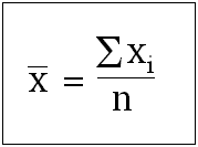
Consider a population with a variable of interest called, "x". If we draw a random sample of size "n", the sample mean of "x" will be given by the following equation.

Now if we have to draw an inference about the population mean of "x", we need to know about the distribution of sample mean of "x". The distribution of any such sample statistic (like sample mean) is known as a sampling distribution (of mean in this case). The Central Limit Theorem (CLT) gives us three very important pieces of information that help us in drawing the required inference.

First, the mean of sampling distribution is equal to population mean. This can be understood intuitively. When we repeatedly sample from the given population, and record the each sample mean, we will observe that (a) it is highly unlikely that the sample means are exactly equal to the population mean, (b) some sample mean will be smaller than the population mean, (c) some sample mean will be larger than the population mean. Now since our sampling is truly random without any bias, the deviations of sampling mean from the population mean in either direction will be equally likely. Therefore, we can conclude that the sampling distribution mean is equal to population mean.

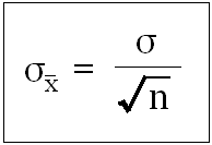
Second, the standard deviation of the sampling distribution is given by the following equation.

This is called "standard error". This can also be understood intuitively. The larger the standard deviation of population, the larger would be sampling error i.e. the standard deviation of sampling distribution. Therefore, standard deviation of population appears in the numerator. In any case, larger the sample size, smaller would be sampling error. This happens because you get a more representative same leading to lesser dispersion in sampling distribution. This is why "n" appears in the denominator. The square root indicates the returns diminish faster with increase in sample size. For example, if you increase a sample size to 40 from 10 (a 4x increase), the standard deviation will only reduce by 1/2 and not by 1/4.

Third, if the sample size is large enough (typically more than 30), the sampling distribution of mean will tend to be distributed normally. This is true irrespective of the distribution pattern of population. This phenomenon seems true intuitively as most of the random natural distributions are normal in nature.

Now armed with this knowledge, we can easily compute the certainty (or uncertainty) in a measurement for a required precision. This certainty (or probability) is called "confidence interval" (CI). Since, the sampling distribution is normal, the computations are very simple. For example for 95% CI for μ is given below:

Just to recap, 95% CI means 95% area under the normal curve or an area covered within 1.96 times the standard deviation (or Z-score, refer to section on Measure of Dispersion) away from the mean in both directions.

And the figure for 99% CI will be

Coming back to correct sample size, note that this depends on (a) variation in population, (b) standard error, and (c) required CI. Typically as rule of thumb, a minimum sample size of 30 is required and in most cases, a sample size between 50 and 100 is good enough.

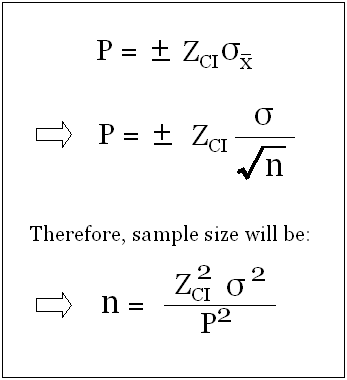
A more formal method can be derived in form of a formula. For a given CI, corresponding Zci can be found in any z-score table. Therefore, as discussed earlier, μ for the given CI will be given by following equation.

We can say that the precision, "P" will be,

Selecting the sampling technique

There are many sampling techniques. This section discusses three key methods.

Simple Random Sampling ensures that each element of the population has an equal chance of being selected. Typically, random number generators are used to select a random sample from the population.

Systematic Random Sampling is a modified form of random sampling. It adds a bit of order to random sampling. The first element of the population is selected randomly. After that, starting from this randomly selected element, every nth element is selected, where n is equal to the population size divided by the sample size. It is easier compared to the simple random sampling. However, it is not suitable if there is a periodicity in the population. It works very well if the list is haphazard.

Stratified Random Sampling is another form of modified random sampling. In this case, the entire population is divided in to homogenous subgroups that share a common characteristic. Thereafter, random sampling is carried out on each group. This technique reduces the standard error and produces more representative sample from the population whenever subgroups are present or possible. For example, if our washers are produced on three different machines then it may be a good idea to have three subgroups (one for each machine) for stratified random sampling.

With this introductory note on sampling, you are now ready to carry out some basic sampling and start drawing inference about the population. More detailed and in-depth discussion will be coming up later.

Commenting Guidelines
We hope the conversations that take place on “discover6sigma.org” will be constructive in context of the topic. To ensure the quality of the discussion stays in check, our moderators will review all the comments and may edit them for clarity and relevance. The comments that are posted using fowl language, promotional phrases and are not relevant in the said context, may be deleted as per moderators discretion. By posting a comment here, you agree to give “discover6sigma.org” the rights to use the contents of your comments anywhere.